
This isn't news to anyone except an absolute spreadsheet beginner. Most folks also know that when you copy and paste a formula that contains cell addresses, Sheets or Excel gives you the relative reference of your target cell. In other words, Sheets/Excel knows that if I copy and paste my formula (=A2) into the cells below (cells C3-C7), I probably don't actually want all of these cells to point to cell A2. If I did really put the formula "=A2" into all of my cells, then I would just get a column cells that all return the same thing

What I really want is the value of the cell directly across from my formula. I actually want the cell reference to change as I copy it down the column, like this:

An Example
Let's imagine you have a list of prices and you want to compute the sales tax on each purchase. I know that the tax rate for my area is 6% and I have a list of transactions. I want to compute the sales tax for each transaction in column E.

"Well, that's easy," you say. "I just multiply the sales tax rate (cell C1) by the sale price (cell D4). Haha!"

That's true, you'll get your sales tax figure. But what happens if you try and copy that formula down the column? Relative References gone wrong, that's what!


The Solution: Absolute References
You can use an Absolute Reference to send this message to Sheets (or Excel; they handle cell referencing the same way). To make sure my formula stays glued to that Sales Tax Factor in C1, I can add some dollar signs to my formula before the C and the 1. You can do this by hand, or by putting your cursor somewhere in the C1 cell address and then hitting the F4 key on your keyboard. It looks like this:

I'm telling Sheets, "This cell is money. I like it, I want to keep it, I don't want it to change." Just remember it this way: dollar signs tell Sheets that your cell reference is money and it shouldn't change. Now look what happens when I copy this new, improved formula down the column:

Accurate tax calculations! Notice how, even at the bottom of my column, the last cell is still pointing at the correct sales tax rate, the 6% entered in cell C1.
Absolute Referencing for Arrays
I covered the tremendously useful VLOOKUP function in a previous article. For VLOOKUP to work properly, though, it needs to be pointed at a 'phone book' of data. Most of the time when you use VLOOKUP, it's really important that you use absolute references for your 'phone book'. If you don't, Sheets (or Excel) will assume you want it to move the phone book each time you copy your formula. Here's what that looks like in practice:

You'll notice above that my VLOOKUP function works most of the time, but it's throwing a few errors at me. The farther down I copy my formula, the more errors I'll see until, eventually, my lookup function will just be returning non-stop #N/As. FAIL! To fix this problem, as you've probably already guessed, I need to add some $s to my phone book. I want to tell Sheets that my phone book is in cells 'Index!A2:G30' and those cells are money, I don't want them to change. I can use either the F4 key or enter the $s by hand, but either way, this is what I want my formula to look like:

Mixed References
This is it, your blackbelt test in Spreadsheet References: the Mixed Reference. Mixed references are best illustrated with another example. Let's say I want Sheets to create a multiplication table for me. For reference, a multiplication table is a grid of cells where the result of each cell is calculated by multiplying the cell in the top row with the corresponding value in the leftmost column. Setting up the skeleton of the table is pretty straightforward:

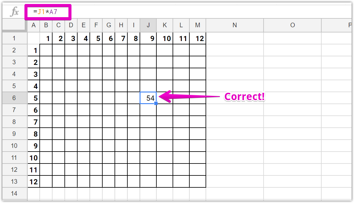
I don't want to write in 144 formulas by hand. Can I copy and paste this =J1*A7 formula to the whole table? (You already know the answer.)

No! And using Absolute References won't work either. Try and guess what will happen if we add those dolla signs to our formula:

Now EVERY cell is multiplying J1 (9) by A7 (6), with predictable results. We need to somehow tell Sheets that we want only a PART of our cell reference to be absolute, and we want the other part to be relative. That's confusing, so we'll break it down in more concrete terms.
Our first cell reference is J1. If we look at our table, we want Sheets to be FIXED in the first row (row 1), but we want it to move between different columns (A-M). We want to send the message: "Yo Sheets, it would be great if you can keep this cell reference fixed up in row 1, but we want the columns to change relative to our formula's location." We do that by adding a $ before the '1' in our cell reference so it reads "J$1":

We aren't done yet because we want the same deal with the other reference (A7). "Hey Sheets! Can you keep this cell reference glued to column A, but I'd like the row (numbers 2-14) to change automatically". We do that by changing our second cell reference to $A7:
Now, watch what happens when we copy THIS formula to our entire table:

Multiplying like a straight-up boss, that's what!
If you didn't catch all of that, don't despair. Mixed references are a difficult beast to master. If you're still confused, I'd suggest actually trying to play around with adding and removing dollar signs (make a copy this sheet as a testing ground). You can also take a look at another article that details this concept. Good luck!